

ANOVA table with SPSS
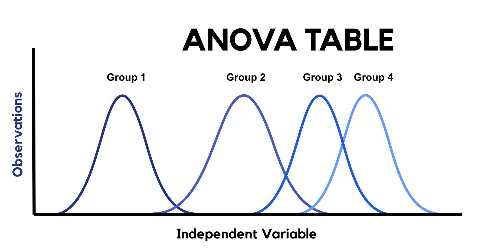
ANOVA or Analysis of Variance is a statistical analysis technique used to compare the means of more than 2 groups, levels or treatments, although its name refers to the study of the observed variability, i.e., 3 or more means are compared based on the dispersion of these means, between groups and within the groups themselves.
A recurrent example of an ANOVA table in Biostatistics would be to corroborate not only the existence of differences between groups as a consequence of the administration or not of a given drug, but also to find out if there is a different effect in terms of, for example, 2 different amounts of the treatment provided.
Índice del Artículo
Outliers Analysis (BOX-PLOT)
First of all, the database itself is purified, discarding outliers that could distort the results of the contrasts and statistical analyses.

Verification of previous hypothesis
Normality
It is checked with the contrasts Kolmogorov-Smirnov-Lilliefors (n>50), Shapiro-Wilk (n<50), and the Asymmetry (near 0 implies normality) and Kurtosis (near 3) tests. The violation of the normality assumption does not significantly affect the Fisher-Snedecor F statistic, provided that the sample sizes are large, because since it is a test of comparative means, the Central Limit Theorem can be applied.
Homocedasticity Verification
Graphical analysis of residues, Bartlett’s Sphericity Test, Hartley Test and the Levene Test of variance homogeneity. The ANOVA is robust against the violation of the homoscedasticity hypothesis, if the sample sizes of the groups or treatments are identical or, at least, very similar.
Independence and randomness of samples Verification: Graphic analysis of waste
The ANOVA Test is not robust against the violation of the hypothesis of independence and randomness of the samples.
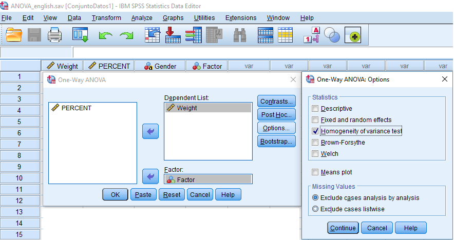
Homocedasticity Test or Variance Homogeneity Test
Ho: Θ12 = Θ12 =…= Θn2
H1: Θi2 <> Θj2 (at least 2 variances are different)
| COCHRAN: Sensitive to discrepancies in Normality, same sample size. |
| BARTLETT (SPHERICITY): Sensitive to discrepancies in Normality, equal sample sizes., Same or different sample size. |
| LEVENE: Less sensitive to discrepancies in Normality than the Bartlett Test, same or different sample sizes. |
The previous hypothesis of homocedasticity cannot be rejected, if the p-value associated with the Levene statistic is greater than 0.05, then the hypothesis of homogeneity of variances of the dependent (response) variable is corroborated, in the groups that conform the independent variable (explanatory) under study.
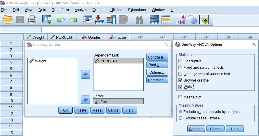
If the Levene test shows that the variances are not significantly homogeneous (that is, the statistically significant resulting contrast), the F statistic is recalculated, selecting the Brown-Forsythe or Welch options box, with which it is carried carry out a transformation of the scores:
ANOVA Oneway Test
Ho (Null hypothesis): The averages of the 3 treatments are equal
Ha (Alternative): Not all means are equal
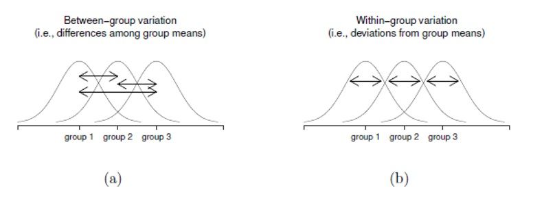

In general, there will be influence of the independent variable or factor (the one that makes up the 3 or more groups), in the continuous dependent variable, if the intergroup variability (between the means of the groups), is greater than the intragroup ( within the groups) or error.
If the Sig. or p-value of the Test is statistically significant (less than 0.05), the null hypothesis that the 3 or more groups behave in the same way with respect to the population mean is rejected, then there are differences in the means of at least 2 groups.
Types of POST-HOC Tests

From Latin ‘after this‘, the Interpretation of the SPSS output results panel is something like that, the crossing of any 2 treatments of the factor whose p-value is less than 0.05 differences are considered statistically significant. If the value of said mean difference is positive, the higher value will be that of the treatment on the left in the comparison, which can also be corroborated with a descriptive analysis of the means, with the submenu command ‘EXPLORE‘. These tests are more robust than performing a Student’s T for comparing means 2 to 2.
Multiple comparison tests are usually based on the probability of at least one Type I error in a set of comparisons. A sort of improved version of Student’s T can be considered for comparisons of population means 2 to 2. The most common Post Hoc tests are:

from Prof. Dr. Tobias Schütz, MBR
Bonferroni
This Post-Hoc multiple comparison correction is used when many statistical tests are performed at the same time. The problem with the execution of many simultaneous tests is that the probability of a significant result increases with each test, for reasons such as that the probabilities of Type II error are high for each test or that it over-corrects Type I errors. This is the test that is usually considered more conservative, widely used in Biostatistics and Psychometrics.
Scheffé method
This test is used when you want to see Post Hoc comparisons in general, (instead of pairwise comparisons). This method is usually taken into account with uneven sample sizes. Very common in non-parametric tests (HSD).
Dunnett
Compare each average with a control average, there is a version for homocedasticity problems.
Tukey
It is based on a number that represents the distance (significant difference) between groups, to compare in this way, each average with each other average of the factor treatments.It is one of the most used a posteriori contrasts assuming homogeneity of variances.
Sidak
Most used in repeated measures ANOVA.
Prueba T2 de Tamhene y Prueba T3 de Dunnett
The most frequently used a posteriori Tests when not starting from equal variances, although in both cases, require compliance with the previous normality hypothesis.